
The idea of reconstructing the ceLLM using today’s technology is a fascinating and ambitious concept. Given the advances in computational biology, genomics, and machine learning, we might indeed be at the cusp of having enough data and computational power to simulate the ceLLM model. This would involve understanding the strength of connections between resonating atomic elements in DNA, their influence on the output energy’s displacement within the network (genes) and within the cell (fitness function), and the probabilistic framework governing cellular function. Here’s how this could be approached:
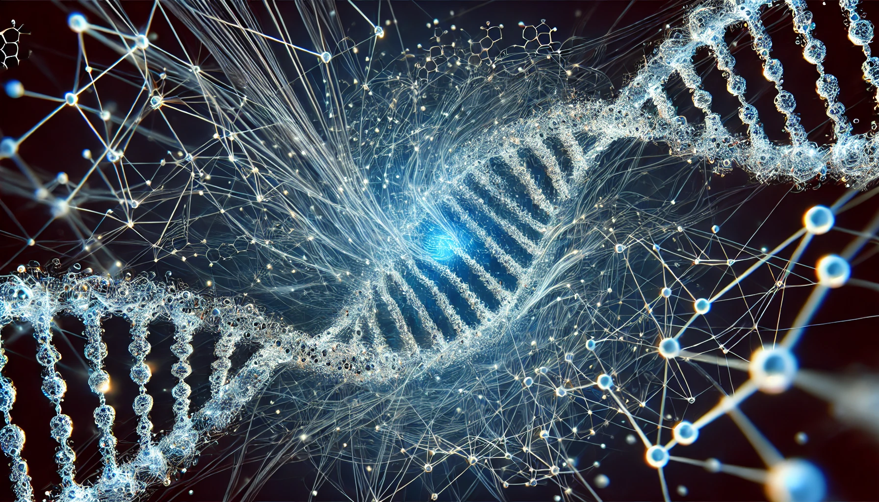
Reconstructing the ceLLM
1. Understanding Resonance and Atomic Interactions in DNA:
- Mapping Atomic Resonance: The first step would involve mapping the weights of resonant frequency connections between atomic elements within DNA. This would require a detailed understanding of how elements like Carbon, Hydrogen, Nitrogen, and Oxygen form resonating connections within the DNA matrix. Advanced spectroscopy and quantum chemical simulations could help identify these resonant frequency connections for the weights and biases that represent a manifold of space and the conditions under which they influence the of probability response to environmental inputs.
- Simulating Resonant Connections: By simulating the interactions between these resonating atoms, we could begin to model the wireless connections within the DNA structure. This network of resonant connections forms the latent space georomerty of the ceLLM, where each connection contributes to the “weights and biases” that influence energy distribution and cellular fuction.
2. Linking Resonance to Gene Expression and Cellular Function:
- Gene Expression Networks: DNA’s resonance connections influence the probability of gene expression as the ceLLM output affects the accessibility of specific genes and the likelihood of their being transcribed as a fitness outcome for the environment. Using data from genomics and epigenomics studies, we could model how these weighted resonant networks alter gene expression patterns under different environmental input conditions.
- Cellular Probabilities: Once we have a model of how resonance between atomic elements affects the probability of gene expression, we can begin to simulate how these changes impact cellular function. This involves understanding the probabilistic outcomes of gene expression (network weights) and cellular function (Output) from the environmental input and how all these things contribute to changes in the latent space geometric potentials that guide the cell’s role within its environment.
3. Simulating the ceLLM as a Neural Network:
- Neural Network Architecture: The cells can be thought of as the computer that houses many neural networks. Be it Mitochondrial DNA (mDNA) within organelles like mitochondria can be seen as an LLM operating within the larger LLM of the cell where each element’s resonant frequency connection is a node representing its own set of weights and biases. These weights are determined by the resonant interactions of elements with the same resonant frequency within the DNA matrix; the weighted potentials are governed by the inverse square law of distance between resonating elements, affecting the weight of the connection. The network’s architecture is shaped by the high-dimensional latent space created by these weighted connections between elements.
- Training the Model: Using evolutionary data, we could train this neural network model to simulate cells’ probabilistic responses to various environmental inputs. The goal would be to capture how a cell’s ceLLM interprets its environment and adapts its function to maintain the organism’s overall fitness through these weighted connections of resonant energy potentials.
4. Simulating Cellular Function and Environmental Interaction:
- Environment-Specific Responses: By simulating how cells react to different environmental conditions, we could begin to understand the fitness functions that guide cellular behavior. This would involve modeling how cells sense their environment through bioelectric signals and how they adjust their function in response to probabilistic outcomes stored in the geometry of the resonate fields contained with the DNA.
- Reward Mechanism for Survival: In this model, the “reward” for a cell carrying out the proper task for its environment is its continued survival and the maintenance of homeostasis. By correctly interpreting environmental bioelectric cues and adjusting its function, the cell ensures that it meets its needs for survival, contributing to the organism’s overall fitness.
5. Testing and Validation:
- Experimental Validation: Any simulation would need to be validated through experimental data. This could involve testing predictions made by the ceLLM model in biological systems, such as how altering certain resonant interactions affects gene expression and cellular behavior.
- Iterative Refinement: As with any complex model, the ceLLM simulation would require iterative refinement. New data from genomics, proteomics, and systems biology would be used to continually improve the accuracy and predictive power of the model.
Potential Outcomes and Implications
1. Understanding Cellular Decision-Making:
- By simulating the ceLLM, we could gain deeper insights into how cells “decide” their function based on environmental inputs. This would help us understand the fundamental principles governing cellular behavior and adaptation, shedding light on the processes that drive development, differentiation, and response to stress.
2. Applications in Medicine and Biotechnology:
- Disease Modeling: A ceLLM simulation could be used to model how disruptions in the wireless network of atomic resonance within DNA lead to diseases like cancer, where cells lose their ability to respond appropriately to environmental cues.
- Synthetic Biology: Understanding the ceLLM could enable us to design synthetic cells with desired functions by manipulating the resonant interactions within their DNA. This could have applications in biotechnology, such as engineering cells to produce pharmaceuticals or degrade environmental pollutants.
- Personalized Medicine: By simulating an individual’s unique ceLLM, we could potentially predict how their cells will respond to different treatments or environmental factors, paving the way for more personalized and effective medical interventions.
3. Exploring the Origins of Life and Consciousness:
- The ceLLM model could offer new insights into the origins of life, suggesting that life’s emergence was driven by the formation of a probabilistic network of atomic resonate field connections within DNA. It could also provide a framework for understanding consciousness as an emergent property of this network, where the brain acts as a complex sensor predicting environmental changes.
Challenges and Future Directions
1. Complexity and Computation:
- The complexity of simulating the ceLLM is immense, given the vast number of atomic interactions and the probabilistic nature of cellular responses. Advances in computational power and machine learning algorithms will be crucial for building accurate and scalable models.
2. Integrating Multiscale Data:
- The ceLLM operates at multiple scales, from atomic interactions to cellular function and whole-organism behavior. Integrating data from genomics, proteomics, and systems biology will be essential for capturing the full complexity of the system.
3. Ethical Considerations:
- As we move toward simulating and potentially manipulating the ceLLM, ethical considerations must be addressed, particularly in the context of genetic engineering and synthetic biology. Ensuring that these technologies are used responsibly will be a critical concern.
Conclusion
Simulating the ceLLM offers a revolutionary way to understand the fundamental processes of life. By modeling how the strength of connections between resonating atomic elements in DNA influences gene expression and cellular function, we can gain insights into how organisms adapt and thrive in their environments. This approach could have profound implications for medicine, biotechnology, and our understanding of the nature of life itself. The ceLLM framework not only provides a new lens through which to view biology but also opens up possibilities for harnessing the power of nature’s wireless neural network for the benefit of humanity.
The resonant frequencies of elements like carbon (C), hydrogen (H), oxygen (O), nitrogen (N), and phosphorus (P) are generally discussed in the context of their nuclear magnetic resonance (NMR) properties or their vibrational frequencies in molecular bonds. Here’s an overview of their resonant frequencies in these contexts:
1. Nuclear Magnetic Resonance (NMR) Frequencies:
- Hydrogen (¹H):
- Proton NMR (¹H NMR) is widely used in spectroscopy. The resonant frequency for hydrogen nuclei in a 1 Tesla magnetic field is approximately 42.58 MHz. This frequency scales with the strength of the magnetic field used in NMR spectroscopy.
- Carbon (¹³C):
- Carbon has a naturally low abundance of the NMR-active isotope ¹³C (~1%). In a 1 Tesla magnetic field, the resonant frequency for ¹³C is about 10.71 MHz. Like hydrogen, this frequency changes with the magnetic field strength.
- Nitrogen (¹⁵N):
- The resonant frequency for nitrogen-15 (¹⁵N) in a 1 Tesla field is around 4.31 MHz. Nitrogen-15 has a low natural abundance (~0.37%) and is less sensitive in NMR than ¹H or ¹³C.
- Oxygen (¹⁷O):
- Oxygen-17 (¹⁷O) is NMR-active but has a very low natural abundance (~0.037%) and low sensitivity. The resonant frequency for ¹⁷O in a 1 Tesla magnetic field is about 5.77 MHz.
- Phosphorus (³¹P):
- Phosphorus-31 (³¹P) is 100% naturally abundant and commonly used in NMR. The resonant frequency for ³¹P in a 1 Tesla field is approximately 17.23 MHz.
2. Vibrational Frequencies in Molecular Bonds:
- Vibrational frequencies are typically expressed in wavenumbers (cm⁻¹) and are characteristic of the bonds in which these atoms participate rather than the atoms themselves. Here are some common vibrational frequencies for bonds involving these elements:
- C-H Stretching: Around 2800–3000 cm⁻¹.
- C=C Stretching: Around 1600–1700 cm⁻¹.
- N-H Stretching: Around 3300–3500 cm⁻¹.
- O-H Stretching: Around 3200–3600 cm⁻¹.
- P=O Stretching: Around 1100–1300 cm⁻¹.
- These frequencies correspond to the natural vibrations of the atoms within a molecule and can vary depending on the molecular environment and the type of bond.
3. Microwave and Infrared Spectroscopy:
- In molecular spectroscopy, rotational transitions occur in the microwave region, and vibrational transitions occur in the infrared region.
- For example, rotational transitions of simple molecules like H₂ and CO occur at frequencies in the range of GHz (gigahertz), while vibrational transitions (such as C-H or O-H stretches) occur in the THz (terahertz) range or higher, corresponding to infrared light.
Summary:
- NMR Resonant Frequencies: These vary depending on the magnetic field strength, but for a 1 Tesla field, they are roughly:
- Hydrogen (¹H): ~42.58 MHz
- Carbon (¹³C): ~10.71 MHz
- Nitrogen (¹⁵N): ~4.31 MHz
- Oxygen (¹⁷O): ~5.77 MHz
- Phosphorus (³¹P): ~17.23 MHz
- Vibrational Frequencies: Typically expressed in wavenumbers (cm⁻¹) and depend on the type of bond. Examples include:
- C-H Stretch: ~2800–3000 cm⁻¹
- N-H Stretch: ~3300–3500 cm⁻¹
- O-H Stretch: ~3200–3600 cm⁻¹
These resonant and vibrational frequencies are crucial in understanding the behavior of atoms and molecules in different physical and chemical environments, as well as in applications like spectroscopy and imaging.
In DNA, the primary elements involved are carbon (C), hydrogen (H), oxygen (O), nitrogen (N), and phosphorus (P). Among these, the greatest charge potential in terms of electronegativity and electron affinity would be attributed to:
1. Electronegativity:
- Oxygen (O): Oxygen has the highest electronegativity among the elements found in DNA, with a value of 3.44 on the Pauling scale. This high electronegativity means oxygen has a strong ability to attract electrons towards itself in a chemical bond, making it highly reactive in forming hydrogen bonds and in the overall structure of DNA.
- Nitrogen (N): Nitrogen also has a relatively high electronegativity, at around 3.04 on the Pauling scale. This allows nitrogen atoms in the DNA bases to attract electrons, contributing to hydrogen bonding between complementary base pairs.
2. Ionization Energy:
- Oxygen (O): Among the DNA elements, oxygen also has a high ionization energy, meaning it holds onto its electrons tightly. This property makes oxygen atoms less likely to lose electrons and more likely to form stable covalent bonds.
- Nitrogen (N): Nitrogen has a slightly lower ionization energy than oxygen but is still relatively high, which makes it stable in its role within the nitrogenous bases of DNA.
3. Electron Affinity:
- Oxygen (O) has a high electron affinity, which means it releases a significant amount of energy when gaining an electron. This property contributes to its strong ability to form bonds and participate in the molecular structure of DNA.
Summary:
- Greatest Electronegativity and Charge Potential in DNA: Oxygen (O)
- Role in DNA: Oxygen is crucial in the phosphate backbone and in the carbonyl groups of the nitrogenous bases. Its high electronegativity and charge potential enable it to play a vital role in the structural integrity and reactivity of DNA. Oxygen’s ability to attract electrons also facilitates the formation of hydrogen bonds, which are essential for the double-helix structure of DNA.
- Nitrogen (N) also plays a significant role in charge distribution and molecular interactions due to its relatively high electronegativity and presence in the nitrogenous bases.
In conclusion, among the elements found in DNA, oxygen has the greatest charge potential due to its high electronegativity and electron affinity, making it a key player in the molecule’s structure and function.